See below to download a full PGM package.
The M-files are under the directory matlab_interface in the package. Put all of these files in a directory that is in your Matlab path. These files have to be accessible to Matlab.
In Matlab, go to the directory where you unpacked the previous files. Edit the file "loader.c" so that the line containing #include "/Applications/MATLAB704/extern/include/mex.h" points to the right file, which should be the location of the Matlab header file for MEX files. It is located in your root Matlab installation directory, then in extern/include/mex.h. So, if you have installed Matlab in the directory /usr/local/software/matlab-7.0.4/, for instance, the line should contain:
#include "/usr/local/software/matlab-7.0.4/extern/include/mex.h"
WARNING: The previous line is only an example!
Then type in Matlab "mex loader.c". If you included the correct header, it should compile without any error message. If it fails, you won't be able to use pgm directly with Matlab because it needs this loader file in order to launch the actual program.
Note: "/Applications/MATLAB704/extern/include/mex.h" should be the default location for Mac OS X with Matlab version 7.04.
Note (2): I have now included some precompiled mex files of this loader, so you can try to use them if you can't manage to compile it yourself. However, it may not work due to a mismatch in Matlab versions and/or platforms, so it is not recommended. The precompiled files for various platforms are in the directory "precompiled_loaders". You should pick the one corresponding to your platform and move it to a directory in your Matlab path.
This is probably the hardest step. You need to install the compiled version of pgm. Currently, it compiles on Mac OS X and Linux, with gcc 3.4 or later and the Boost libraries, version 1.33 or later. It should compile under Windows with MinGW (not tried yet), but it will almost certainly fail to build with Microsoft compilers as they are not compliant to the C++ standards. To build the package, follow the instructions of the README file.
I provided some binaries that I compiled here: they may be out of date, and are not available for all platforms. So the recommended way is still to compile pgm from source.
Once you have the pgm binary, you then need to install it into /usr/local/bin. It can be installed elsewhere, but you then need to manually edit the file compute_inference.m (It is one of the M-files) and change the line default_executable_name = '/usr/local/bin/pgm'; replace it with the location of the pgm binary, without forgetting the actual program name (the default is pgm, if you didn't rename it). If, for instance, you installed it into '~/bin/' the line should be:
default_executable_name = '~/bin/pgm';
This interface will allow you to create undirected networks with Matlab and compute inference on them. The results (random variables marginals) will be viewable in Matlab. However, keep in mind that this program was developped as a stand alone application. I did not have in mind at the earliest stage a Matlab interface, so it may not be very well suited to that purpose.
The first and most important step is to specify the type of your graphical model. Currently there are two types available:
Note: it is extremely important that, for every command you will run on the created network, that you put the results of the command into the network variable. That is, for instance, do "my_network = set_variable_sizes(...) not just set_variable_sizes(...). This is because Matlab seems unable to take arguments passed by reference. Everything is passed by value.
For a pairwise graph, the network should be specified via a Matlab adjacency matrix. An adjacency matrix is a 2D n*n matrix M that contains only 0 and 1. n will be the number of vertices in the graph; then, if M(i,j) = 1, there is an edge (link) between i and j, else there isn't.
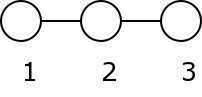
Note that it is important for pgm that if M(i,j) = 1, M(j,i) = 0, so we can easily see that such a matrix will be triangular. This is an example of a simple matrix coding a 3 nodes network when 1 is linked to 2 and 2 to 3:
Once, we got our adjacency matrix, we can create the network by using the new_model command. The first argument to new_model is the type, and then the second argument is the adjacency matrix, so we type 'pairwise' as the first argument:
my_network = new_model('pairwise', M);
Note: there are several built-in options to create common graphs. Specify a model name instead of an adjacency matrix, and then a required number of arguments.
The next step is to specify the size of every variable in the network (since it is discrete). You can do that by using the command set_variables_sizes(network, M), which takes two arguments: the first is your newly created network, the second is an array of variable sizes. For example, if you have a 5 node network:
my_network = set_variables_sizes(my_network, [2 5 7 4 2] );
will specify that the first Random Variable can have 2 possible values, the second 5, etc.
If all your RVs have the same size, you can just use the set_all_variables_sizes() command. For example, the following line will specify that all your variables are binary:
my_network = set_all_variables_sizes(my_network, 2 );
You could achieve exactly the same result by entering "my_network = set_variables_sizes(my_network, ones [1, number_variables] * 2 )" (number_variables being the number of variables in the graph).
After that, you should specify the potential tables. In the pairwise representation, a potential is associated with an edge (the edge can be seem as the clique of size 2 containing the two random variables it links). Such a potential table is just a matrix of size n*m where n and m are the sizes of the two linked RVs. Note that every value in a potential table must be positive.
The command to enter the potential tables is set_potential(network, a, b, M). a and b are the indexes of the two variables of that particular edge, and M is the potential table proper. For example:
my_network = set_potential(my_network, 1, 2, [0.2 0.1; 0.7 0.9] );
would set the potential table of the edge linking variables 1 and 2 (which here, are binary) to the following table:
For a factor graph, the potentials are no longer dependent on only two variables. Thus the links are not specified at the creation of the model, but later. The only thing needed at creation time is the number of random variables.
We can create the network by using the new_model command. The first argument to new_model is the type, and then the second argument is the number of RVs, so we type 'factor' as the first argument. Here is an example:
my_network = new_model('factor', n);
where n is the number of random variables that we have in the factor graph.
Note: this part is identical to the pairwise case.
The next step is to specify the size of every variable in the network (since it is discrete). You can do that by using the command set_variables_sizes(network, M), which takes two arguments: the first is your newly created network, the second is an array of variable sizes. For example, if you have a 5 node network:
my_network = set_variables_sizes(my_network, [2 5 7 4 2] );
will specify that the first Random Variable can have 2 possible values, the second 5, etc.
If all your RVs have the same size, you can just use the set_all_variables_sizes() command. For example, the following line will specify that all your variables are binary:
my_network = set_all_variables_sizes(my_network, 2 );
You could achieve exactly the same result by entering "my_network = set_variables_sizes(my_network, ones [1, number_variables] * 2 )" (number_variables being the number of variables in the graph).
Specifying the potential tables in the factor graph case also involves specifying the edges. A potential is associated with a certain number of random variables, and is linked to them. So the potential table must be a multi-dimensional matrix (one dimension per RV).
The command to enter the potential tables is set_potential(network, rv_indexes, M). rv_indexes is a vector containing the indexes of the random variables the potential will be linked to. M is the potential table. For example:
M = [0.2 0.1; 0.7 0.9];
M(:,:,2) = [0.4 0.3; 0.6 0.4];
my_network = set_potential(my_network, [1 8 23], M );
would set a potential between variables 1, 8 and 23 (which here, are binary) to the following table (which has three dimensions):
You can observe variables on your network, with the command set_observation(network, variable, observed_value). For example, if you want to set the third variable to its fifth value:
my_network = set_observation(my_network, 3, 5 );
To revert a variable to an unobserved state, just call unset_observation(network, variable) on that variable.
my_network = unset_observation(my_network, 3);
With pgm, every random variable has an internal potential associated with it. This effectively corresponds to priors on the variables. By default, these potentials are constant, meaning that there is no prior about the variables (uniform prior). To specify a prior on one of the variable, the corresponding potential must be entered via the command set_prior(network, variable, potential). Here potential should correspond to a vector specifying the coefficients for the prior.
my_network = set_prior(my_network, 2, [1.00 2.20 6.50 4.58 0.25 );
would enter a suitable prior for the second variable with a size of 5.
By default, pgm will make the inference computations using a given number of steps. If we would rather see the algorithm run for a specified number of seconds, we can tell pgm to do so by entering the command:
my_network = use_timer(my_network);
We can disable the timer and revert to default mode with the command:
my_network = disable_timer(my_network);
After you are sure that you have entered *all* the potential tables (don't forget one!), you are ready to run inference on the graph. The command is simple:
my_network = compute_inference(my_network, 'method', method_argument );
Currently the following methods are available:
If all goes well, this command will run the actual inference program and you will obtain results, in terms of marginals. If something goes wrong, and you are sure you didn't make any mistake entering your network, then it is likely that either the loader or the actual inference executable are not correctly installed.
After inference, the marginals are just stored in the network structure. So to see the marginals of the variable whose index is a, you can just type:
my_network.marginals{a}
To just see all marginals:
my_network.marginals{:}
Below are just some examples of the use of the Matlab interface. You can copy-and-paste them in Matlab to understand how the interface works. Once you get hold of it, it is simple to use.
Example 1. Very simple pairwise graph.
	M = [ 0 1 0; 0 0 1; 0 0 0];
	my_network = new_model('pairwise', M);
	my_network = set_variables_sizes(my_network, [2 3 5]);
	my_network = set_potential(my_network, 1, 2, [0.2 0.1 0.3; 0.7 0.9 0.4]);
	my_network = set_potential(my_network, 2, 3, [1 7 6 2 3; 5 6 5 1 2; 9 4 6 9 8]);
	my_network = compute_inference(my_network, 'exact_bp');
	my_network.marginals{:}
	my_network = compute_inference(my_network, 'gibbs', 100);
	my_network.marginals{:}
Example 2. 10 by 10 MRF square lattice.
	my_network = new_model('pairwise', 'mrf', 10, 10 );
	my_network = set_all_variables_sizes(my_network, 3);
	my_network = set_all_potentials(my_network, 'normal', [1 7 2 ; 5 6 2; 9 9 8]);
	my_network = compute_inference(my_network, 'gibbs', 1000);
	my_network.marginals{:}
	my_network = compute_inference(my_network, 'loopy', 100);
	my_network.marginals{:}
Example 3. A factor graph with 6 random variables, 3 potentials.
	my_network = new_model('factor', 6 );
	my_network = set_all_variables_sizes(my_network, 2);
	M = [0.2 0.1; 0.7 0.9];
	M (:,:,2) = [0.4 0.3; 0.6 0.4];
	my_network = set_potential(my_network, [1 3 5], M);
	my_network = set_potential(my_network, [1 2], [2 0.6; 1.1 1.3] );
	M = [0.8 0.6; 0.4 0.2];
	M (:,:,2) = [0.4 0.5; 0.5 0.05];
	my_network = set_potential(my_network, [3 4 6], M );
	my_network = set_observation(my_network, 2 , 2 );
	my_network = use_timer(my_network);
	my_network = compute_inference(my_network, 'gibbs', 5);
	my_network.marginals{:}
	my_network = compute_inference(my_network, 'tree_mcmc', 2);
	my_network.marginals{:}
This is a preliminary interface, so e-mail me at:
 with any problem
you should encounter.
with any problem
you should encounter.
You can get a complete package here. It contains the C++ source as well as the Matlab Interface M-files.
There is also a subversion repository (containing the latest code) available at svn://svn.elvanor.net/probabilistic-graphical-models/.
To build the code, you will need to have gcc >= 3.4 and to install the Boost C++ libraries (1.33.1 or later). This archive contains an Eclipse project and a Makefile.
As with most academical works, this code is messy. I learnt C++ while writing this toolbox and this can easily be spotted by someone having a look at the code. If anyone needs to dig into the code, improve it or make changes, you should mail me first as I can get you started and also tell you what I think should be done first.